Featured article. Pages 1, 2, 3.
Normal And Anomalous Osmosis Through A Leaking Membrane
THE PHYSICS AND PHYSIOLOGY OF OXYGEN: AN INTERDISCIPLINARY APPROACH TO EXPLAIN OXYGEN TRANSPORT TO ISHEMIC / HYPOXIC TISSUE IN HYPERBARIC OXYGEN TREATMENT
A. Babchin1, E. Levich1, Y. Melamed2, G. Sivashinsky1
1Tel Aviv University, Tel Aviv 69978, Israel, 2Hyperbaric Medical Center, Elisha and Rambam Hospitals, Haifa, 34636, Israel
***For the Firefox web browser: to make sure you see the scientific characters correctly, please select on the Firefox toolbar: View menu-->Character Encoding-->Unicode (UTF-8)***
Kylstra et al.[8] provided an experimental example of the osmotic pressure and flow through leaking membrane induced by concentration gradient of a gas (nitrous oxide) dissolved in water. For accuracy we cite the original authors: "The pressure in an osmometer filled with nitrous oxide- saturated water separated from water by a polyurethane polyether membrane 2.5 microns in thickness, rose slowly by 8 to 20 millimeters (of water) in ten minutes before gradually returning to close to zero within two hours." "It is concluded that dissolved gases exert osmotic pressure. Partial pressure gradients of dissolved gases in the tissues of animals and man should cause flows of water along osmotic gradients, which may partially account for some of the symptoms and signs of dysbarism."
The provided description of experimental results indicates two time scales of osmotic flow and solute transport through porous membrane:
- Short time osmotic flow of the solvent with correspondent convective solute transfer, and,
- Long time molecular diffusion of solute leading to the equilibrium state.
Interpreting the observed data in the language of physicochemical hydrodynamics [9], a standard equation of convective diffusion quantifies the solute flux within porous membrane:
|
|
(1) |
Where J is the molar flux of the solute (moles/sec cm3 ), C is the solute concentration, D is the solute diffusion coefficient inside porous membrane, x is the coordinate in the direction normal to the membrane surface.
The averaged velocity v of the liquid within the porous membrane is expressed by Darcy law:
|
|
(2) |
K denotes the membranes absolute permeability to the hydrodynamic flow, µ is the viscosity of liquid, Posm is the difference in osmotic pressures between two sides of membrane, L is membrane width, Á is the fluid density, g is the gravity acceleration constant and H is the height of hydrostatic column caused by osmotic pressure and observed as the difference in the position of the liquid-gas surfaces in compartments separated by the membrane. Evidently, the osmotic pressure and the gravity head, induced by hydrostatic column, act in opposite directions.
It should be noted, that the origin of osmotic pressure exerted by leaking membranes in the case of non-electrolyte solute is due to the long range molecular forces and was first explained by Derjaguin in 1947. This subject was further developed by Derjaguin, Dukhin and Churaev in numerous publications. Osmotic pressure for a non-electrolyte solution (oxygen dissolved in water is an example) can be determined locally in the vicinity of solid surface as follows [10, 11, 12],
|
|
(3) |
Where C (z) is the solute concentration within the diffuse adsorption layer and C0(mol/cm3) is the bulk solute concentration beyond the adsorption layer, R is gaseous constant and T is absolute temperature. In the case of dilute solutions, the concentration of solute molecules in the field of long range molecular forces is expressed by the Boltzmann distribution:
|
|
(4) |
Here k is the Boltzman constant, and U(z) is the energy of a solute molecule at the distance z from the solid surface. The value of U(z) is negative if a solute molecule experiences attraction to the surface. In this case the concentration of solute molecules near solid-liquid interface exceeds their concentration in the bulk of the solution. However, if the solid surface repels solute molecules the value of U(z) is positive, rendering the concentration deficit of the solute near the solid surface or within porous body.
In the case of high specific surface of porous media, which corresponds to small pore sizes, the diffuse adsorption (desorption) layers overlap. With strongly overlapping diffuse molecular layers the difference between the energies of solute molecules within this layer can be assumed much smaller than the characteristic value U of solute molecules near the interface. This approximation was initially applied for the description of osmotic flow in electrolyte solutions by Babchin and Frenkel [13].
Incorporation of the characteristic value of molecular interactions U, allows rewriting Eq.(4) as:
|
|
(5) |
Combining Eqs.(3) and (5) results in the following relation for the osmotic pressure:
|
|
(6) |
In the case of small molecular energies U/kT << 1, Eq.(6) becomes:
|
|
(7) |
Having two values of bulk concentration, one in each compartment, separated by a membrane, the osmotic pressure difference driving the fluid through membrane may be written as:
|
|
(8) |
C20 and C30 denote the solute bulk concentrations on each side of the membrane. With Eqs.(2) and (8) taken into account, the Darcy velocity v within porous membrane reads:
|
|
(9) |
Guided by the experimental data provided by Kylstra et al. [8], it is assumed that commence- ment of the osmotic transport process is dominated by the convective term. The solvent flows from the low concentration to the higher solute concentration compartment. The volume conservation requirement for incompressible fluid allows expression of the rate of change in the observed hydrostatic column in terms of the Darcy velocity as:
|
|
(10) |
where B1 is the dimensionless constant, determined by the osmotic cell geometry. With v determined by Eq. (9), the following differential equation describes H(t) behavior at the beginning of the process:
|
|
(11) |
Considering the concentration difference as a constant at the beginning of the process, the solution of Eq.(11) can be represented as:
|
|
(12) |
Where K1 = ÁgB1K/µ > 0, K2 = (B1K/µ)(U/kT)(C30 - C20).
The hydrostatic column H(t) marks the difference between liquid levels in the compartment with higher concentration of the solute C3 and in the compartment with the lower solute concentration C2. The case of normal osmosis assumes the fluid flow through porous membrane to be directed from lower to higher solute concentration. Under these conditions the values of H(t) should be positive. The coefficient K1 in the Eq.(12) is always a positive constant.
Thus, the direction of flow depends on the sign of K2. With (C3 - C2) > 0, the effect of normal osmosis will take place and will be observed at U > 0. Positive energies of the solute molecules near the membrane surfaces signify that these molecules experience repulsion in the vicinity of the membrane material. On the contrary, when membrane material surfaces attract solute molecules, their energy U < 0, the coefficient K2 becomes negative, rendering a negative sign for the hydrostatic column H(t).
Experimental observation will exhibit the depression of the liquid level in the compartment with higher concentration C3 of the solute and elevation of the liquid level in the compartment with lower solute concentration C2. Observation of this kind leads to the irrefutable conclusion that osmotic flow is directed from the higher to lower solute concentration values and is directed opposite to the solute concentration gradient.
Since the direction of flow in this case is opposite to one in normal osmosis this phenomenon is historically called anomalous osmosis. There is nothing anomalous in the attraction of the solute molecules to interfaces and the terminology is rather archaic, having its root in times when only semi permeable membranes were tested for osmotic phenomena. Experimentally the anomalous osmosis in leaking membranes was observed long before theoretical explanations [14].
The fast process of solution transport by convection, caused by osmotic pressure gradient, recedes in time when the hydrostatic column reaches its maximum. At this time moment osmotic flow is opposed by a counter flow caused by gravity head, so that the actual total flow of liquid through the membrane is zero. The solute transport experiences reversal (in the case of normal osmosis) since it is governed by slow molecular diffusion and directed from higher to lower solute concentration. The time dependent molecular flux of the solute at this stage can be expressed as:
|
|
(13) |
where D is the diffusion coefficient of the solute within porous membrane. At the first approxima- tion D may be expressed (accounting for the porosity (Æ) and tortuosity (Ä ) of porous membrane), as D = (Æ/Ä )Dbulk.
As transport of the solvent through the membrane is much faster than one of the solute, the relaxation of H(t) to zero will be controlled by the molecular diffusion of the solute. As the concentration difference between compartments decreases, the column H(t) decreases as well. The osmotic pressure, which characterizes H(t), will experience the consequence of steady states controlled by a concentration difference at a given moment of time.
Thus, only the molecular flux, described by Eq.(13) along with initial concentrations and cell geometry affect the characteristic time of relaxation process. Considering osmotic cell as having two equal compartments, each of volume V , the equation for the solute mass conservation becomes:
|
|
(14) |
and:
|
|
(15) |
where A is the membrane area separating two compartments. The initial condition for Eq.(15) is: C3 - C2= C30 - C20, which yields the solution,
|
|
(16) |
In the discussed consequence of steady states Eq.(8) can be extended to the time dependent expression for the osmotic pressure difference:
|
|
(17) |
which determines the momentary value of the gravity head ÁgH(t). Thus,
|
|
(18) |
The time dependent solution for the experimentally observed hydrostatic column during the overall process time may be represented by asymptotic matching of Eqs.(12) and (18). The matching can be performed through the conventional procedure [15], provided that the typical time-scale L/K1 of Eq.(12) is much smaller than the time-scale LV/AD of Eq.(18). In this case the long-time limit of H(t) governed by Eq.(12) should coincide with the short-time limit of H(t) governed by Eq.(18). Hence,
|
|
(19) |
where Nav is the Avogadro number. The expression for H(t), uniformly valid over the entire time interval, then reads:
|
|
(20) |
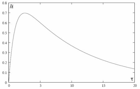
Figure 1. Temporal evolution of the hydrostatic column height (scaled).
Figure 1 plots the scaled height h = H/Q versus scaled time Ä = K1t/L at AD/VK1 = 0.1. Combining Eqs.(19) and (20), the final result for H(t) as a measurement of time dependent osmotic pressure reads:
|
|
(21) |
As a conclusion to this physicochemical part of the paper, is should be noted that similarity with normal and anomalous osmosis can be found in the diffusiophoreses, the phenomenon reciprocal to the capillary osmosis. This similarity is well explained by Anderson, Lowell and Prieve [16]:When a particle is placed in a fluid in which there is a non-uniform concentration of solute, it will move toward higher or lower concentration depending on whether the solute is attracted to or repelled from the particle surface.
Numerical example: at the oxygen concentration difference in blood plasma and tissue of 60mg/L = 2.10(-6)mol/cm3, and assuming rather strong molecular interaction between the oxygen and tissue with U = 0.5(kT ), the resulting osmotic pressure, calculated from Eq.(21) at maximum H(t) comes to 24cm of water column. This value drops to about 5cm at U = -0.1kT.
For PDF version of this article click here...
Sponsored links: